Lecture 10
THE INCOME-EXPENDITURE DIAGRAM

1. Aggregate expenditure vs. GDP

• Recall: AE = C + I + G + (X-IM)

• Case 1: AE < Y
  With spending below ouput, inventories will start to climb.
  Firms will then cut back on production, causing Y to decrease.

• Case 2: If AE > Y
  Firms will produce more output (why?)

2. Equilibrium condition in the goods market

• Aggregate spending equals output
• Y = AE
• Y = C + I + G + (X-IM)

3. Model #1 (The base model)

• Objective: To determine the eqbm level of GDP in the economy

3.1 Assumptions

1. Consumption (C)
   • C increases with disposable income
   • C = a + b(Y-T)
   • Recall the parameters for the consumption function

2. Investment (I)
   • Assumed to be exogenous
   • Level of investment is fixed

3. Government spending (G)
   • Assumed to be exogenous
   • Level of govt. spending is fixed

4. Net exports (X-IM)
   • Assumed to be exogenous
   • Level of net exports is fixed

5. Taxes (T)
   • Assumed to be fixed

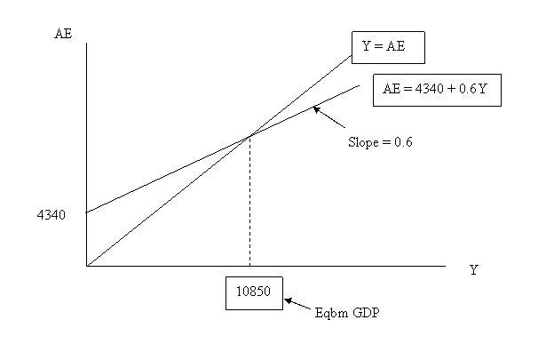
3.2 Income-Expenditure diagram

Step 1: Plot aggregate expenditure vs. GDP
Step 2: Plot 45-degree line through the origin
Step 3: Obtain the eqbm level of GDP

3.3 Analytical solution

Step 1: Obtain the expression for aggregate expenditure (AE) in terms of Y
Step 2: Use the condition for eqbm in the goods market: Y = AE
Step 3: Solve for Y

3.4 Equilibrium consumption

• Graphically: Read off the value from the consumption function
• Analytically: Substitute the value of Y in the consumption function

3.5 Equilibrium saving

• Derive the saving function (in terms of GDP)
• Recall: S = DI - C

3.6 Example

Consider the following model of an economy:

C = 2000 + 0.6DI
T = 100
I = 800
G = 1200
X-IM = 400

Fig. Income–Expenditure Diagram

4. Relationship between S and I

• Recall: S = I + (G-T) + (X-IM)

4.1 Special cases

• Case 1: No government; No trade (closed economy)
  G = 0, T = 0; X = 0, IM = 0

• Case 2: Closed economy
  X = 0, IM = 0

5. Model #2

5.1 Assumptions

• Same as in Model #1, except that Imports are endogenous
• Import demand function: IM increases with GDP
• Marginal Propensity to Import (MPM): Coefficient of GDP
• Example: IM = 500 + 0.1Y

5.2 Income-expenditure diagram

• Slope of the AE-line is no longer equal to MPC
• Slope equals: MPC - MPM

5.3 Equilibrium

• Obtain eqbm values of: Y, C, S, Net Exports